Use Kari's AI agent to analyze the correlation between the unit-area price of second-hand condominiums and other variables

Copyright © 2026GotoAI Inc.Based on the goose project

Verification environment

The steps on this page were verified in the following environment.

• Kari: version 0.7.3, Windows
• AI provider: OpenAI ChatGPT subscription
• Model: GPT-6.1 Sol High

About this page

On the previous page we learned which columns hold what, and in what proportions. What we want to know next is what prices move together with.

We build Y = transaction price (total) ÷ area (m²), that is, the price per square metre, and make it the axis of the analysis. And we narrow the target to second-hand condominiums (「中古マンション等」). As we saw on the previous page, three quarters of the records are second-hand condominiums, and their prices are set differently from land and from land with a building (detached houses). Look at correlations with the types mixed, and you end up seeing differences between types rather than relationships with the variables.

On that basis, we measure the strength of the relationship between Y and each of the remaining 26 variables. The difficulty here is that the measure to use depends on the type of the variable.

Type of variable	Measure	Range	Sign
Numeric (building age, distance to station, etc.)	Pearson's r	−1 to 1	Yes (+ for increasing, − for decreasing)
Categorical (municipality name, layout, etc.)	Correlation ratio η	0 to 1	No

Sorting 26 variables by type, using the right measure for each, ranking them, and then looking inside the top variables is a day's work by hand. We have the AI build this whole sequence in one go as a Kari Dataflow.

Preparing the work

• Check that 「データコレクション1:不動産価格.csv:テーブル1」 (Data Collection 1 : real estate prices CSV : Table 1), created on the previous page, is registered in the Data Collection.

• Open a chat session. As on the previous page, creating the Dataflow starts from an instruction in the chat.

Instruct the AI

• Give the extraction conditions, the formulas for the variables to create, and the names of the Dataflows to save, all in one instruction. The prompt below is an English rendering of the Japanese prompt shown in the screenshot; table, column, value and dataflow names are quoted as they appear in the Japanese source data.

Prompt for the AI

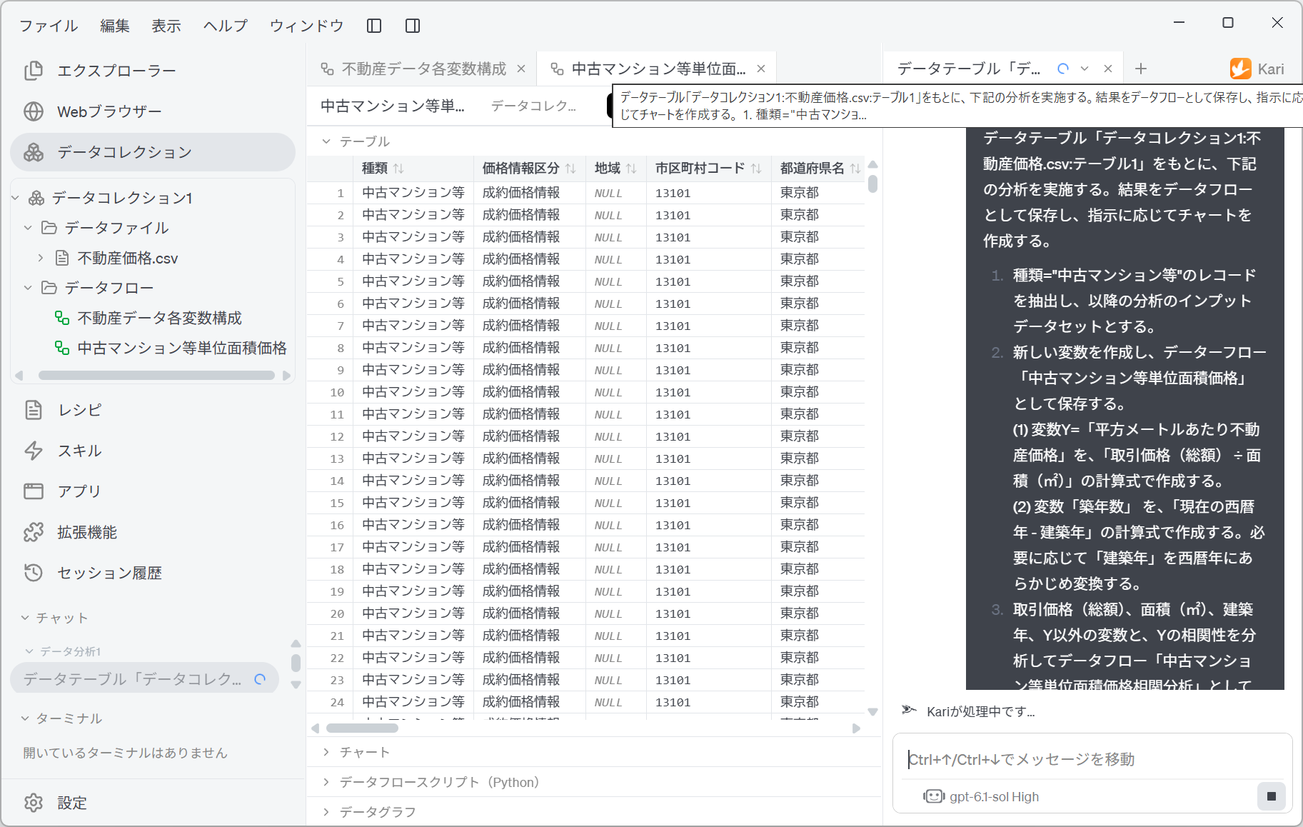
Based on the data table 「データコレクション1:不動産価格.csv:テーブル1」, carry out the analysis below. Save the results as dataflows and create charts as instructed.

1. Extract the records where 種類 = "中古マンション等", and use them as the input dataset for the rest of the analysis.
2. Create new variables and save them as the dataflow 「中古マンション等単位面積価格」.
  (1) Create the variable Y = 「平方メートルあたり不動産価格」 (real estate price per square metre) with the formula 「取引価格（総額） ÷ 面積（㎡）」.
  (2) Create the variable 「築年数」 (building age) with the formula 「現在の西暦年 - 建築年」 (current Western calendar year − year built). Convert 「建築年」 to a Western calendar year beforehand if necessary.
3. Analyze the correlation of Y with the variables other than 取引価格（総額）, 面積（㎡）, 建築年 and Y, and save the result as the dataflow 「中古マンション等単位面積価格相関分析」. If a correlation could not be analyzed, state the reason in the chat.
4. In the correlation results, add a flag classifying each variable as categorical or numeric, and add the rank of the strength of correlation within each class.
5. For the categorical variables and for the numeric variables, create two column charts each, shown in descending order of the absolute value of the correlation.
6. Choose the top three categorical variables by strength of correlation, and for each create a column chart showing the Y value, in descending order of Y. Explain the correlation measure in the chart's note.
7. Choose the top three continuous numeric variables by strength of correlation, and for each create a scatter plot with that variable on the horizontal axis and Y on the vertical axis. Explain the correlation measure in the chart's note.

Screenshot shown in the original Japanese.

The way this instruction is put together has a few key points.

Block of the instruction	What it is for
1. Narrow by type	Fixes the population for the analysis first. With the types mixed, you measure the difference between types rather than correlations with the variables.
2-(1) Definition of Y	Gives the calculation as a formula, not in words. Write only "unit-area price", and whether it is per m² or per tsubo, a total or a price per m², is left to the AI's interpretation.
2-(2) Definition of building age	Writing "convert 建築年 (year built) to a Western calendar year beforehand if necessary" puts the preprocessing into the instruction too. 建築年 is a string such as 1990年, and some rows use Japanese era years.
3. State which variables to exclude	Two kinds of variable are excluded, for different reasons. 取引価格（総額） (transaction price, total) and 面積（㎡） (area, m²) are the very ingredients of Y; if they are not excluded, the top of the list fills up with the obvious result that they correlate strongly with Y. 建築年 is the same information as building age (building age = base year − year built); leave it in, and the same information takes two places at the top of the ranking.
3. Report when analysis is impossible	The instruction says "if a correlation could not be analyzed, state the reason in the chat". Not letting anything drop silently is what makes the later checking possible.
4. Class flag and rank within class	Keeps the ranking intact even though measures of different kinds (r and η) sit in one table. With the rank within class, numeric and categorical variables can be read separately.
5. Two charts per class	"Two each" means four charts in all. The absolute value shows the ranking by strength, the signed value shows the direction. The same measure is presented in two views.
6-7. Drill into the top three variables	A ranking only tells you that something "has an effect". Limiting it to looking inside only the top variables avoids waste such as plotting all 843 levels. The instruction to explain the measure in the note is attached here too.
Naming the Dataflows	Intermediate results are given names and saved. Later analyses can refer to them as input.

caution

Always include the instruction to exclude the variables Y is made from. Since Y = price ÷ area, if transaction price (total) is not excluded, its correlation comes near the top simply because of how the variable is defined — but that is not the real-world relationship you want to know about.

Check the AI's work

• The AI carries out the extraction, the creation of variables, the correlation analysis and the charts all at once, and reports the result.

Screenshot shown in the original Japanese.

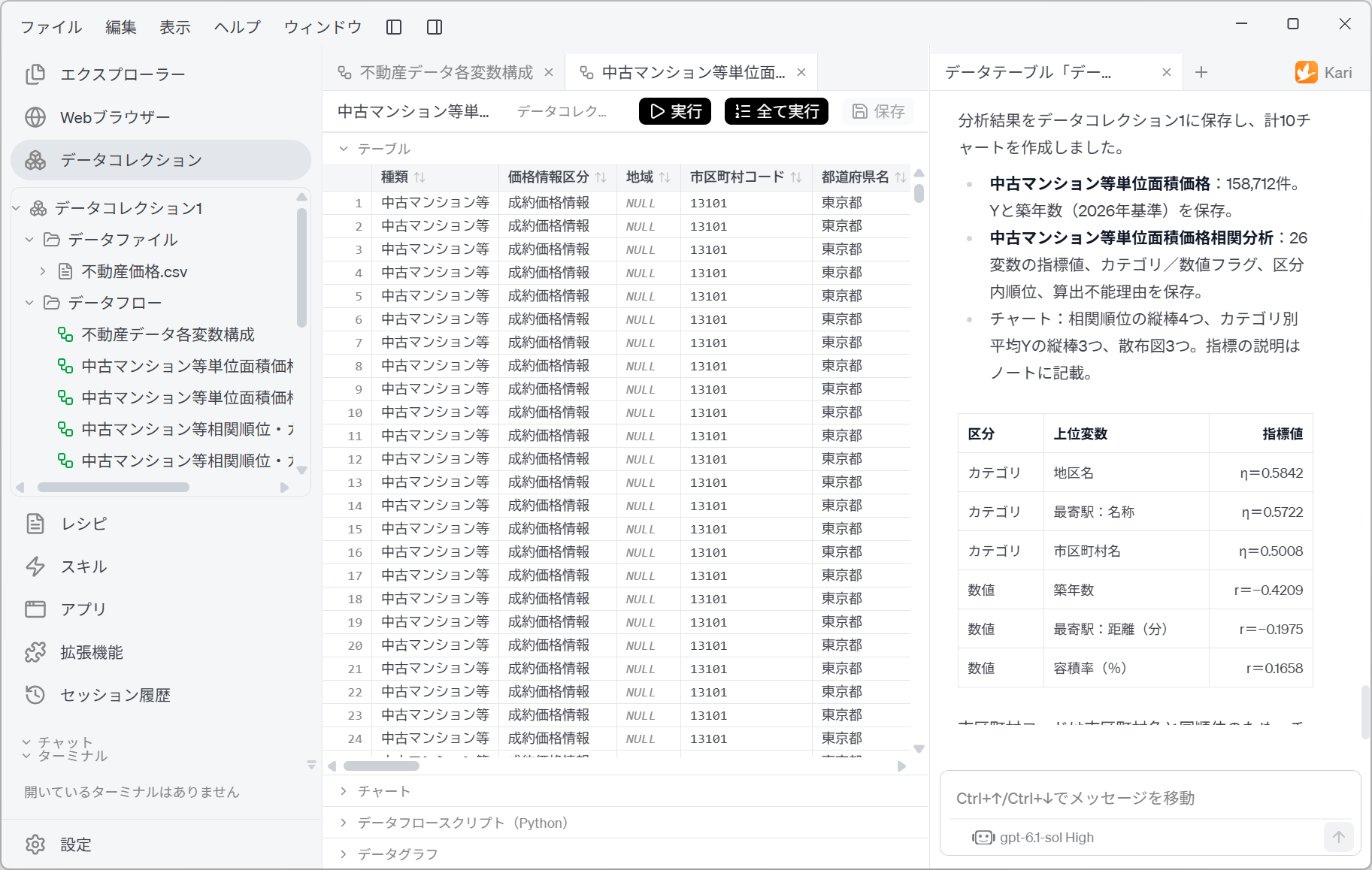
In this example, the AI reports the following.

• 中古マンション等単位面積価格 (unit-area price of second-hand condominiums): 158,712 records. Y and building age (as of 2026) are saved.
• 中古マンション等単位面積価格相関分析 (correlation analysis of the unit-area price of second-hand condominiums): the measure for each of the 26 variables, the categorical/numeric flag, the rank within class and the reason a measure could not be calculated are saved.
• Charts: four column charts of the correlation ranks, three column charts of average Y by category, and three scatter plots, ten charts in all. The explanation of the measures is in the notes.

Class	Top variable	Measure
Categorical	地区名 (district name)	η=0.5842
Categorical	最寄駅：名称 (nearest station: name)	η=0.5722
Categorical	市区町村名 (municipality name)	η=0.5008
Numeric	築年数 (building age)	r=−0.4209
Numeric	最寄駅：距離（分） (nearest station: distance (minutes))	r=−0.1975
Numeric	容積率（％） (floor area ratio (%))	r=0.1658

• At the end of the report, the AI adds a caution about how to read its own result: "because 市区町村コード (municipality code) has the same rank as 市区町村名". This points out that the same classification is held in two columns — a place where, reading the ranking from the top, you would count the same information twice. The other duplicate pair, year built and building age, does not appear here because this time year built was excluded at the instruction stage.

• In addition, the variables that could not be analyzed are reported by name. In this example: 「地域、土地の形状、間口、延床面積、前面道路の方位・種類・幅員」 (area type, land shape, frontage, total floor area, and the frontage road's direction, type and width). This is because land and frontage road information is hardly ever recorded for second-hand condominiums; it is not missing data but the nature of the data.

The reason a variable could not be analyzed remains as a column

The generated script writes a reason for each variable that could not be analyzed: "no valid values of the variable in rows where Y is valid", "the variable has only one value, so variance is zero", "fewer than two valid pairs". Which variables dropped out, and why, is kept as data, not as text in the chat.

Look at the strongly correlated variables by rank

• First, the numeric variables. They are sorted in descending order of the absolute value of Pearson's r.

Screenshot shown in the original Japanese.

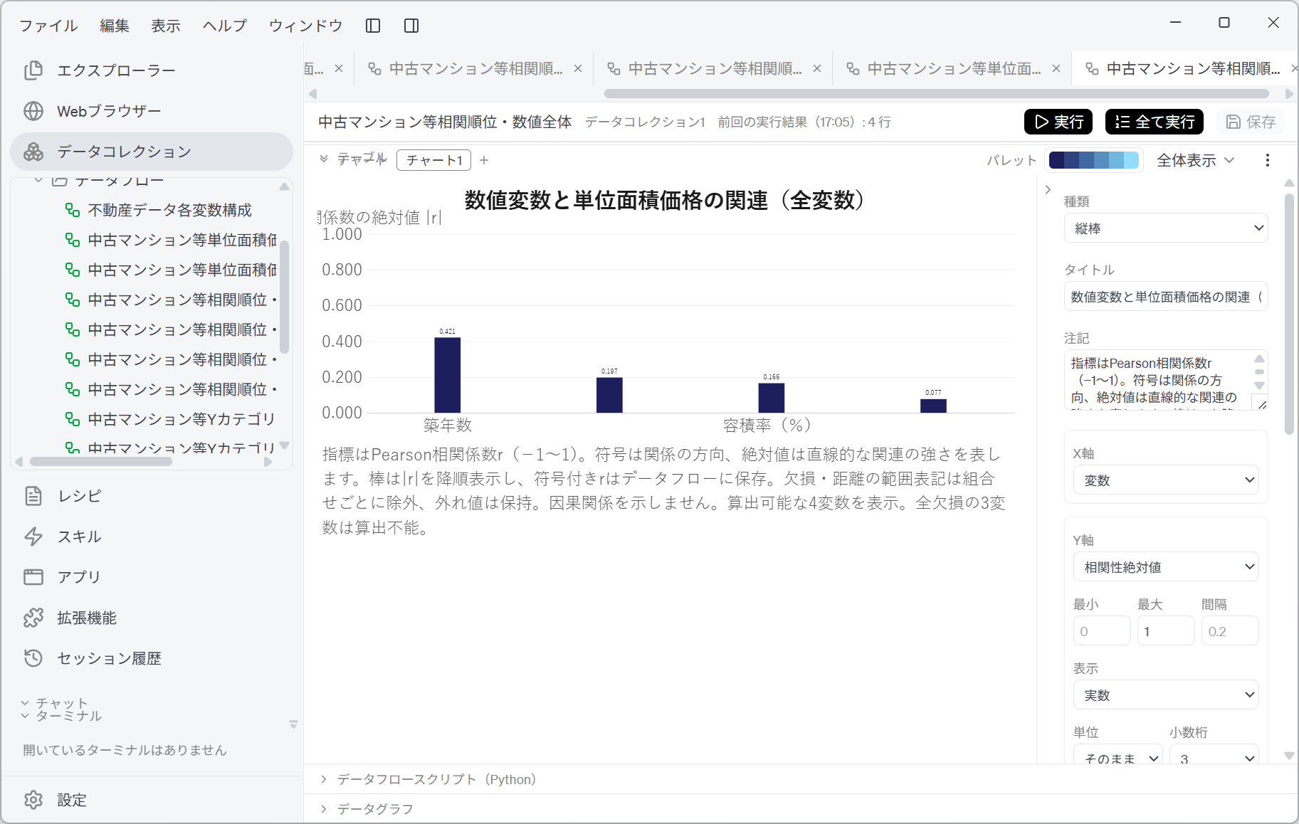
Building age, at 0.421, is a head above the rest, followed by nearest station: distance at 0.197, floor area ratio at 0.166 and building coverage ratio at 0.077. There are only four bars. The note at the bottom of the chart states the assumptions, including the reason.

The measure is Pearson's correlation coefficient r (−1 to 1). The sign shows the direction of the relationship, the absolute value the strength of the linear association. Bars show absolute values in descending order; signed r is saved in the dataflow. Missing values and range notations for distance are excluded pair by pair; outliers are kept. Does not show causation. The 4 variables that could be calculated are shown. The 3 variables that are entirely missing could not be calculated.

There were seven numeric variables, but frontage, total floor area and frontage road: width are missing in every record for second-hand condominiums, so the measure could not be calculated at all. A missing bar means not that the value is small but that there is no data.

• Next, the categorical variables. They are sorted in descending order of the correlation ratio η.

Screenshot shown in the original Japanese.

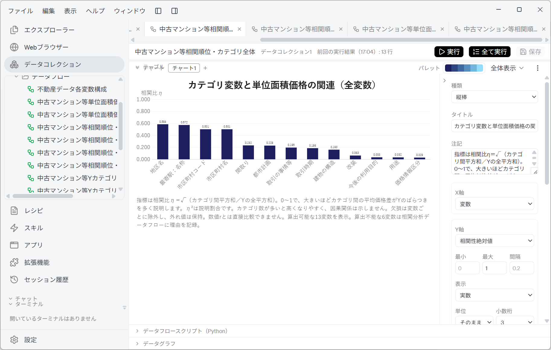
District name at 0.584 and nearest station: name at 0.572 are at the top, with municipality code and municipality name level at 0.501. They are followed by layout (間取り) at 0.232, city planning (都市計画) at 0.228, circumstances of the transaction (取引の事情等) at 0.195, transaction period (取引時期) at 0.186 and building structure (建物の構造) at 0.160; renovation (改装), intended future use (今後の利用目的), use (用途) and price information category (価格情報区分) are at 0.063 or below. The 13 variables that could be calculated are shown, and for the 6 that could not, the reasons are recorded in the Dataflow.

Two cautions written in the note

It tends to be higher when there are many categories, and does not show causation. (omitted) It cannot be compared directly with the numeric r.

The first. District name may be in first place because the district really does have an effect — or it may be because district name has as many as 843 levels. The more finely you cut the categories, the smaller the spread within each group, and the higher η goes. The ranking of categorical variables has to be read together with the number of levels.

The second. η and r are different measures, and you must not compare their sizes. You cannot set district name's η=0.584 beside building age's r=−0.421 and conclude that "the district has more effect". The AI produces two separate charts precisely so that these two are not put on the same axis.

Look at average Y by category

A ranking only tells you that something "has an effect". Now look at which values are high and which are cheap.

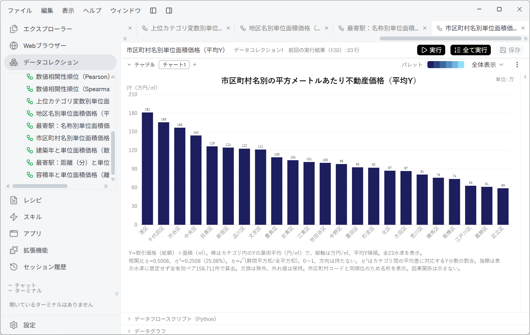
• Average Y by municipality name. All 23 wards are shown.

Screenshot shown in the original Japanese.

Minato Ward leads at 1.81 million yen/m², followed by Chiyoda Ward at 1.65 million, Shibuya Ward at 1.56 million and Chuo Ward at 1.44 million; at the bottom is Adachi Ward at 590,000 yen/m². The highest is about three times the lowest.

The note says η=0.5008, η²=0.2508 (25.08%). η² is "the share of the variance of Y that corresponds to differences in means between categories", so it reads as: the ward alone explains about a quarter of the variation in price per m².

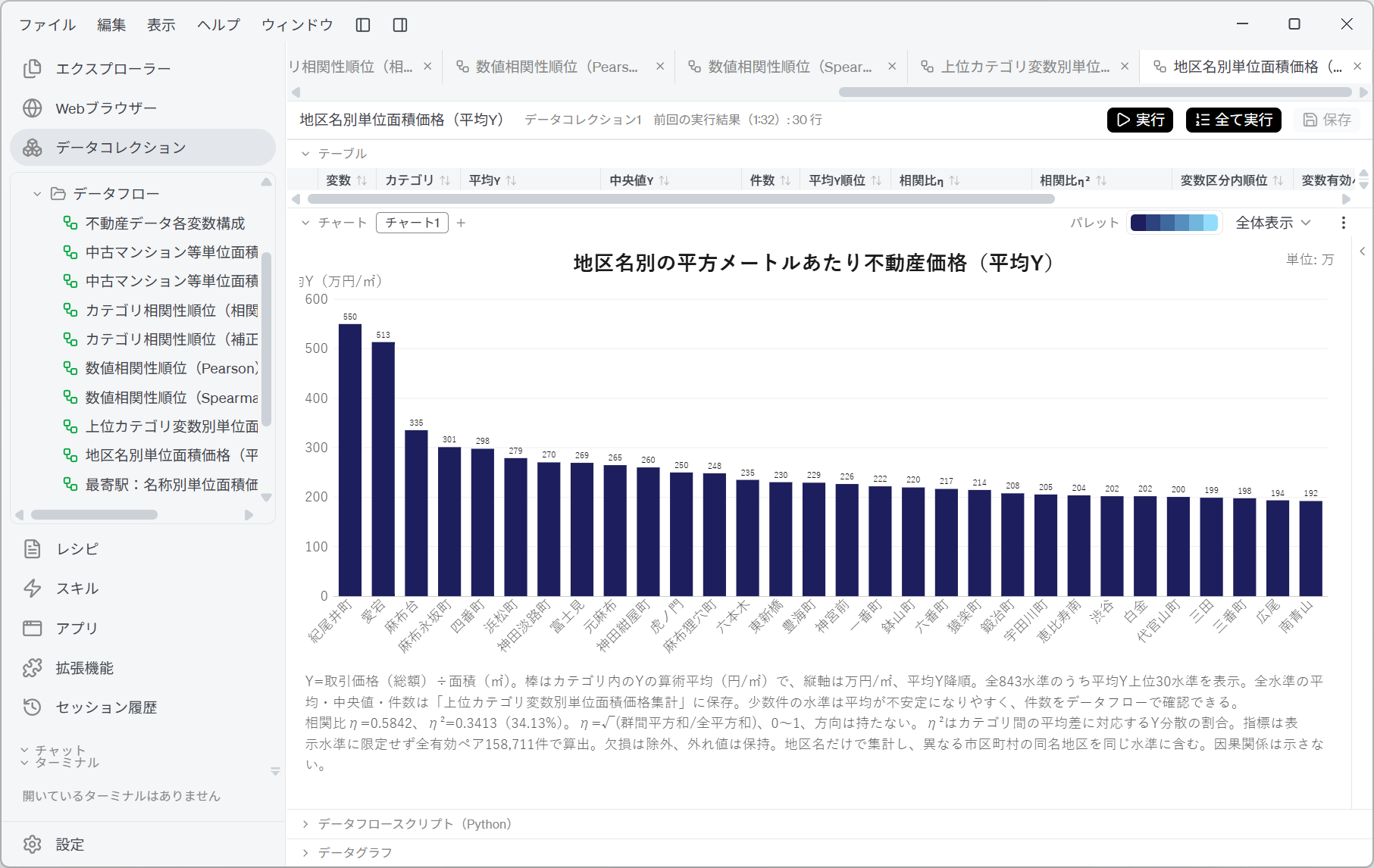
• Average Y by district name. Because there are so many levels, only the top 30 are shown.

Screenshot shown in the original Japanese.

Kioicho (紀尾井町) at 5.5 million yen/m², Atago (愛宕) at 5.13 million, Azabudai (麻布台) at 3.35 million — the spread is far larger than for municipality name. η² is 34.13%, above municipality name's 25.08%.

Three assumptions written in the notes of these two charts

1. Only the top 30 of all 843 levels are shown. The remaining 813 are not on screen. The mean, median and count for every level are saved in a separate Dataflow.
2. The mean is unstable for levels with few records. A district with only a handful of records may be at the very top. You can check the counts in the Dataflow.
3. The aggregation is by district name alone, so districts with the same name in different municipalities are counted as the same level. District names such as 「本町」 (Honcho) and 「中央」 (Chuo) exist in several wards.

Check the shape of the relationship in scatter plots

A correlation coefficient squashes the shape of a relationship into a single number. The same r=0.4 may be a clean straight line or may bend part way. For the top numeric variables, look at the shape in a scatter plot.

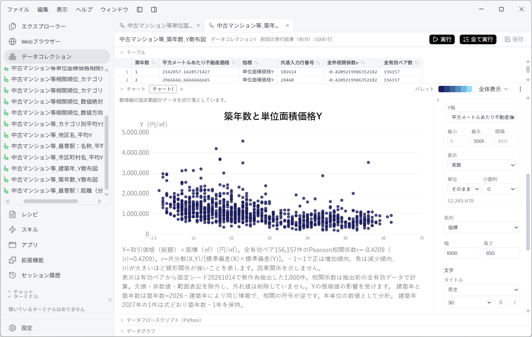
• Building age and Y.

Screenshot shown in the original Japanese.

r=−0.4209 (156,157 valid pairs in all). The tendency for the unit price to fall as building age rises can be read in the spread of the points too. But the spread is wide at the newer end, which also shows that building age alone does not determine the price.

The points displayed are 1,000 records drawn at random from the valid pairs with the fixed seed 20261014. The correlation coefficient was calculated on all the valid data before sampling, so although the display is a sample, the measure is for all records.

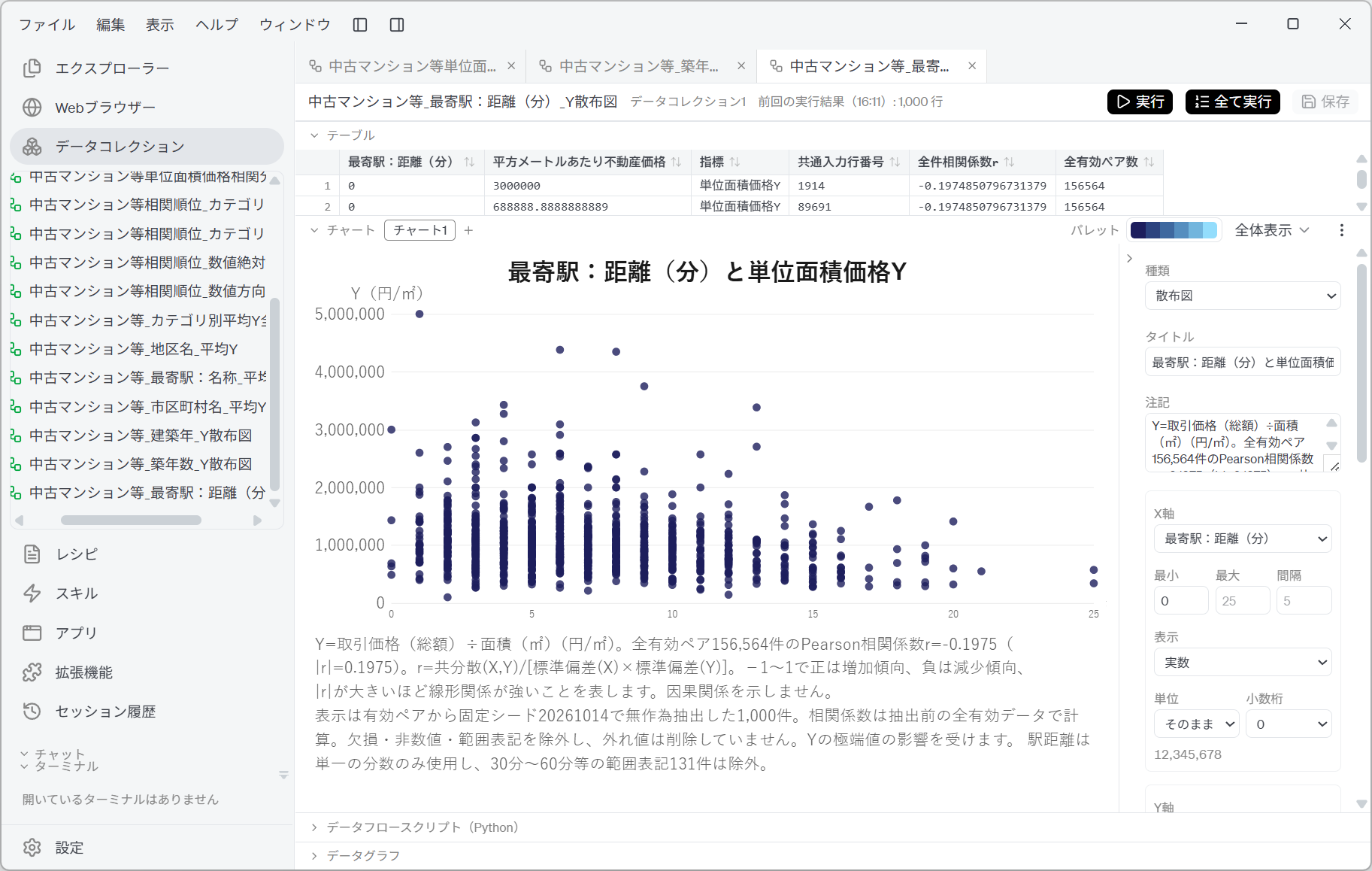
• Nearest station: distance (minutes) and Y.

Screenshot shown in the original Japanese.

r=−0.1975 (156,564 valid pairs in all). There is a tendency for prices to be lower further from the station, but it is not as clear as with building age.

The note carries an important proviso.

For station distance only single minute values are used; 131 range notations such as 30 to 60 minutes are excluded.

This is the notation problem mentioned on the overview page. Replacing 「30分〜60分」 (30 to 60 minutes) or 「1H〜1H30」 (1 hour to 1 hour 30) with, say, 45 or 75 minutes would add points, but it would create precision that does not exist. The AI did not assume a representative value; it excluded these records and stated how many.

What you notice when you look at the scatter plots

In both scatter plots, the points are cut off at the upper limit of the vertical axis. If the chart shows the notice "The fixed axis range cuts off some of the data.", there is real data above the upper limit of the axis. Whether to look at everything including outliers, or to fix the range and look at the dense part of the distribution, is up to your purpose.

Human-in-the-loop points

Do not leave everything to the AI. Check the following yourself.

• Check that the same information is not counted twice
  Municipality code and municipality name are the same classification, and their η is identical. You think you have taken the top four, but in effect you are looking at only three variables. Year built and building age are also the same information, since 築年数＝基準年−建築年 (building age = base year − year built), but here this was avoided by excluding year built at the instruction stage. In the first run both appeared in the ranking, and two scatter plots were even drawn. Preventing duplicates in the instruction is the reliable way.

• Do not compare sizes across measures
  The correlation ratio η and Pearson's r are different measures. The chart's note also says "it cannot be compared directly with the numeric r". You cannot set district name's η=0.584 beside building age's r=−0.421 and say "the district has more effect".

• Read the ranking of categories together with the number of levels
  The correlation ratio η comes out higher for variables with more levels. That district name (843 levels) ranks above municipality name (23 levels) does not necessarily mean that the district has more effect. A table ranked by η alone, without evening out the number of levels, is built so that the most finely cut variable wins.

• Look at the counts behind the averages
  The top 30 by district name are in descending order of average Y. The average of a district with only a few records moves up and down easily. For the top districts, check the counts in the Dataflow before using them in a conclusion.

• Read the ranking itself with the bases evened out
  The number of rows usable differs from variable to variable. In this example, 取引の事情等 (circumstances of the transaction) is in seventh place (η=0.195), but it has only 334 valid pairs out of 158,711. Renovation with 63,437, use with 59,392, and floor area ratio and building coverage ratio with 70,605 are also less than half of the total. Read the chart with the understanding that variables whose bases differ by two orders of magnitude sit in the same bar chart.

• Do not judge on the correlation coefficient alone — look at the scatter plot
  r squashes the shape of a relationship. A scatter plot shows not only the strength of the tendency but also how wide the spread is. Building age's r=−0.42 should be read not as "building age determines the price" but as "there is a tendency, but it alone does not determine the price".

• Check the number of rows excluded
  The 131 range notations for station distance, rows where area is given as a range, rows where year built is 「戦前」 (pre-war) — all of these were excluded. Excluding them is the right decision, but the fact that they were excluded is information that should accompany the conclusion.

• Do not reread it as causation
  Every chart's note says "does not show causation". That unit prices are high in Minato Ward is not the same as their being high because it is Minato Ward. Correlation is a tool for deciding what to investigate next, not a conclusion.

caution

The choice of measure, the sorting of variables and the composition of the charts can vary with the LLM used. Which variable was measured with which measure must always be checked in the Dataflow's 「変数区分」 (variable class) column.

References

The data analyzed on this page was obtained from the Real Estate Information Library (「不動産情報ライブラリ」) of the Ministry of Land, Infrastructure, Transport and Tourism. Screenshots are reproduced as quotations with the source stated. The correlation measures, rankings and charts that the AI produced were generated by GotoAI as an example of Kari's operation; they were not created or published by the Ministry of Land, Infrastructure, Transport and Tourism.

• Material: Real Estate Information Library (「不動産情報ライブラリ」), 「不動産価格（取引価格・成約価格）情報の検索・ダウンロード」 (search and download of real estate price information: transaction prices and closed-sale prices)
• Provider: Ministry of Land, Infrastructure, Transport and Tourism (MLIT)
• URL: https://www.reinfolib.mlit.go.jp/realEstatePrices/
• Accessed: October 13, 2026
• Terms of use: Subject to that site's terms of use. Source: MLIT website (URL above).

For the nature of the data (that it is based on a questionnaire survey, that transaction prices are rounded to two significant figures, and that two sources are mixed), see "The nature of the data" in the Overview.

Disclaimer

• The external information quoted on this site is provided to illustrate examples of using Kari. This site does not guarantee the accuracy or currency of that information. Quoted sources may be changed or removed without notice.
• The AI output shown on this site was actually obtained in the stated verification environment. However, this site does not guarantee the accuracy or usefulness of that output. AI output varies with the LLM used, its settings, and from one run to the next.
• The correlation measures on this page were calculated under the stated assumptions (narrowing to second-hand condominiums, keeping outliers, excluding missing values pair by pair). If the assumptions change, the values change too.
• Correlation does not show causation. None of the figures on this page identifies what determines prices.
• Screenshots were taken with the version of Kari current at the time of writing. The display may differ in your version.
• This page deals with data on actual real estate transaction prices. If you use it for purchase or investment decisions, always check it against the original data.
• The organizations quoted have no affiliation with, and do not endorse, this site or Kari.